BitFunnel performance estimation

First, I’m going to talk about one way to think about performance. That is, one way you can reason about performance.

In case it’s not obvious, this is a psuedo-transcript of a talk given at StrangeLoop 2016. See this link if you’d rather watch the video. I wrote this up before watching my talk, so the text probably doesn’t match the video exactly.

However, when applications get larger, most applications become performance sensitive! This happens both because making a large application faster reduces its cost, and also because making a large application faster can increase its revenue. The second part isn’t intuitive to many people, but we’ll talk more about that later.

But when I look at outcomes, well, I often see two applications designed to the same thing that were implemented with similar resources where one application is 10x or 100x faster than the other. And when I ask around and find out why, I almost inevetiably find that the team that wrote the faster application spent a lot of time on design. I tend to work on applications that take a year or two to build, so let’s say we’re talking about something that took a year and a half. For a project of that duration, it’s not uncommon to spend months in the design phase before anyone writes any code that’s intended to be production code. And when I look at the slower application, the team that created the slower appliction usually had the idea that “meetings and whiteboarding aren’t real work” and jumped straight into coding.
The problem is that if you have something that takes a year and a half to build, if you build it, measure the performance, and then decide to iterate, your iteration time is a year and a half, whereas on the whiteboard, it can be hours or days. Moreover, if you build a system without reasoning about what the performance should be, when you build the system and measure its performance, you’ll only know how fast it runs, not how fast it should run, so you won’t even know that you should iterate.
It’s common to hear advice like “don’t optimize early, just profile and then optimize the important parts after it works”. That’s fine advice for non-performance critical systems, but it’s very bad advice for performane critical systems, where you may find that you have to re-do the entire architecture to get as much performance out of the system as your machine can give you.
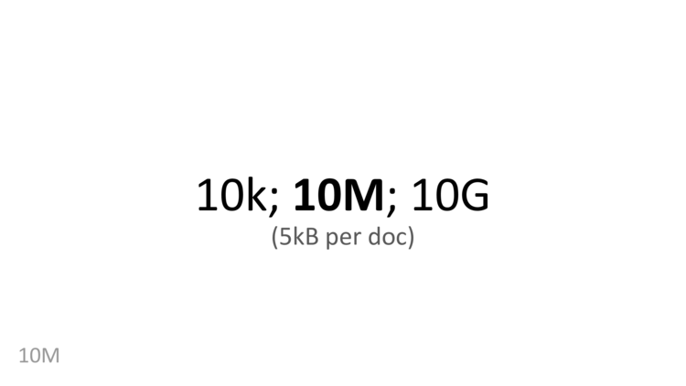
And let’s assume that each document is 5kB. If we’re talking about the web, that’s a bit too small, and if we’re talking about email, that’s a bit too big, but you can scale this number to whatever corpus size you have.
AND queries.

AND yellow AND dog. The systems we’ll look at today can handle ORs and NOTs, but those aren’t fundamentally different and talking about them will add complexity, so we’ll only look at AND queries.

k times a k is a million, and five times time is fifty, so 5kB times ten thousand is 50MB.

50MB is really small!

1GB of RAM. 50MB will easily fit in RAM, even on a low-end phone.
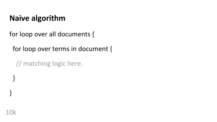
50MB, we can try the most naive thing possible and basially just grep through our data. If you want something more concrete, you can think of this as looping over all documents, and for each document, looping over all terms.
Since we only need to handle AND queries, we can keep track of all the terms we want, and if a document has all of the terms we want, we can add that to our list of matches.

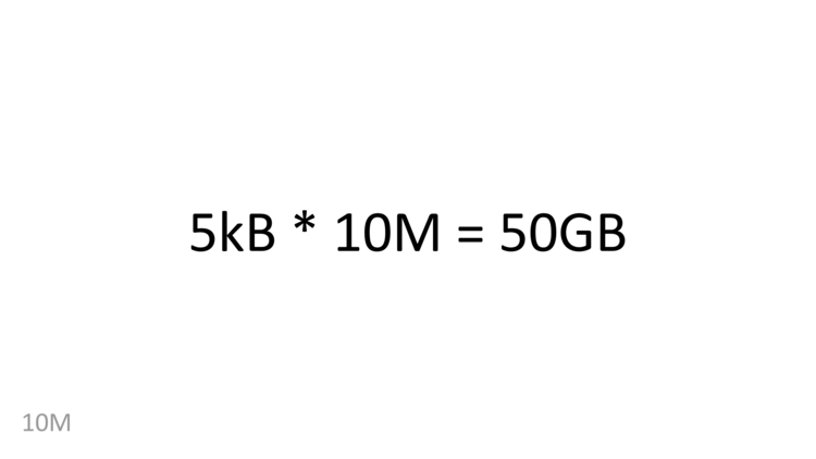
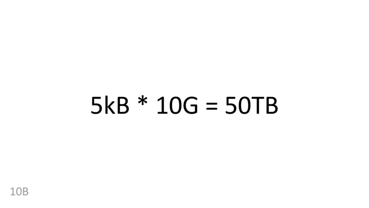
5kB times ten million is 50GB. This is really close to wikipedia’s size – today, wikipedia is a bit over 50GB (uncompressed articles in XML, no talk, no history).

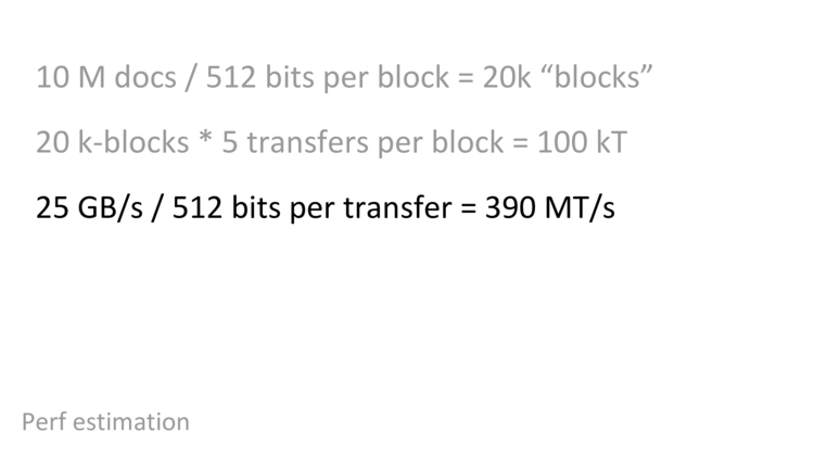
25GB/s of bandwidth…
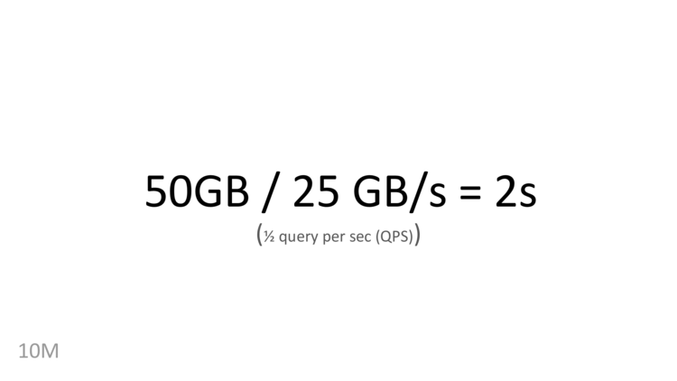
And while we’re doing a query, we’re using all the bandwidth on the machine, so we can’t expect to do anything else on the machine while queries are running, including other queries. This implies that it takes two seconds to do a query, or that we get one-half a query per second, or 1⁄2 QPS.
For many applications, that’s totally fine! I know a lot of devs who have an internal search tool (often over things like logs) that takes a second or two to return results. They’d like to get results back faster, but given the cost/benefit tradeoff, it’s not worth optimizing things more.
As with latency, a lot of devs I know have a search service that’s only used internally. If you have 10 or 20 devs typing in queries at keyboards, it’s pretty unlikely that they’ll exceed 1⁄2 QPS with manual queries, so there’s no point in creating a system that can handle more throughput.
Our naive grep-like algorithm is totally fine for many search problems!
Amazon found that every 100ms of latency cost them more than 1% of revenue. Google once found that adding 500ms of latency, or half a second, cost them 20% of their users.
This isn’t only true of large companies – when Mobify looked at this, they also found that 100ms of latency cost them more than 1% of revenue. For them, 1% was only $300k or so. But even though I say “only”, that’s enough to pay a junior developer for a year. Latency can really matter!
That’s a lot of stuff! If you do budgeting for a service like this and you want queries to have a half-second end-user round-trip budget, you’ll probably only leave tens of milliseconds to handle document matching on the machines that recieve queries and tell you which documents matched the queries. Two seconds of latency is definitely not ok in that case.
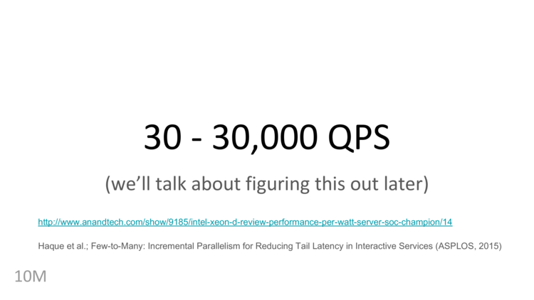
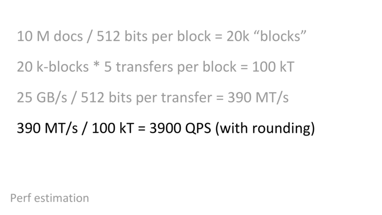
Today, we’ll talk about how to get performance in the range of thousands to tens of thousands of queries per second, but first…
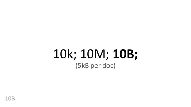
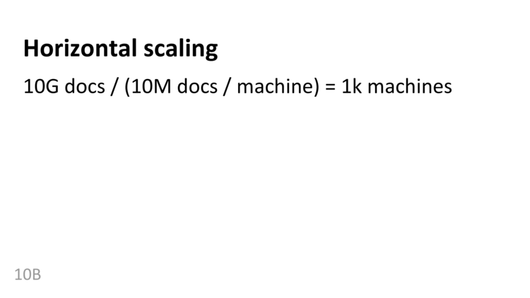
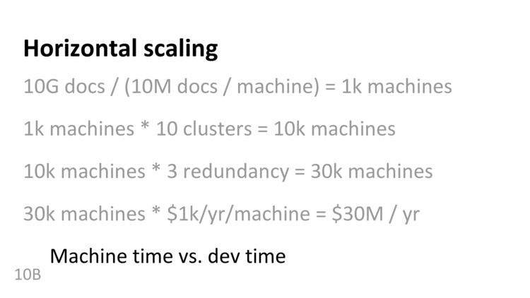
We’ve said that we can, using some kind of index, serve ten million documents from one machine with performance that we find to be acceptble. So how about ten billion?
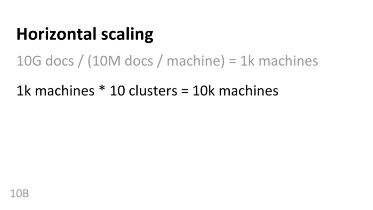
That’s ok, but if we have a cluster of a thousand machines and the cluster is in Redmond, and we have a customer in Europe, that could easily add 300ms of latnecy to the query. We’ve gone through all the effort of designing and index that can return a query in 10ms, and then we have customers that lose 300ms from having their queries go back and forth over the internet.
Instead of having a single cluster, we can use multiple clusters all over the world to reduce that problem.
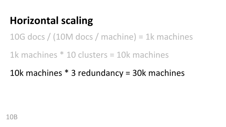
With ten thousand machines (or even with a thousand machines), we have another problem: given the failure rate of commodity hardware, with ten thousand machines, machines will be failing all the time. At any given time, in any given cluster, some machines will be down. If, for example, the machine that’s indexing cnn.com goes down and users who want to query that cluster can’t get results from CNN, that’s bad.
With thirty thousand machines, one problem we have is that we now have a distributed system. That’s a super interesting set of problems, but it’s beyond the scope of this talk.
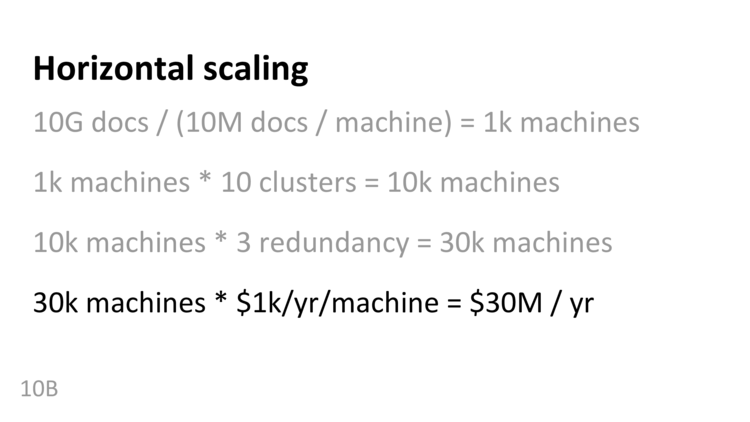
At thirty-million a year, if we can double the performance and halve the number of machines we need, that saves us fifteen-million a year. In fact, if we can even shave off one percent on the running time of a query, that would save three-hundred thousand dollars a year, saving enough money to pay a junior developer for an entire year.

AND queries.


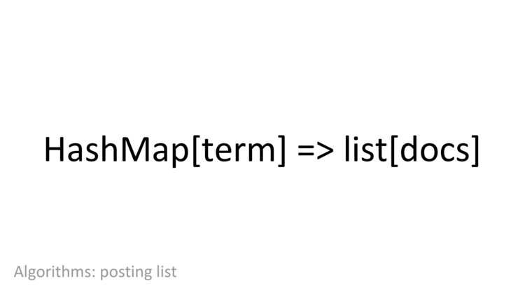
Here’s an index from the 1600s. If you look at the back of a book today, you’ll see the same thing: there’s a list of terms, and next to each term there’s a list pages that term appears on.
Computers don’t have pages in the same sense; if you want to imagine a simple version of a posting list, you can think of…
One thing we might try would to be use something called in incidence matrix, that is, a 2d matrix where one dimension of the matrix is every single term we know about, and the other dimension is every single document we know about. Each entry in the matrix is a 1 if the term is in the document, and it’s a 0 if the term isn’t in the document.
What will the performance of that be?
pause
someone shouts ten million
In fact, if you limit the search to just github, you can find a single document with about fifty-million primes! And if you look at the whole internet, you can find a site with all primes under one trillion, which is over thirty-billion primes! If that site lands in a single shard, that shard is going to have at least thirty-billion unique terms. Turns out, a lot of people put long mathematical sequences online.
And in addition to numbers, there’s stuff that’s often designed to be unique, like catalog numbers, ID numbers, error codes, and GUIDs. Plus DNA! Really, DNA. Ok, DNA isn’t designed to be unique, but if you split it up into chunks of arbitrary numbers of characters, there’s a high probability that any N character chunk for N > 16 is unique.
There’s a lot of this stuff! One question you might ask is, do you need to index that stuff? Does anyone really search for GTGACCTTGGGCAAGTTACTTAACCTCTCTGTGCCTCAGTTTCCTCATCTGTAAAATGGGGATAATA?
It turns out, that when you ask people to evaluate a search engine, many of them will try to imagine the weirdest queries they can think of, try those, and then choose the search engine that handles those queries better. It doesn’t matter that they never do those queries normally. Some real people actually evaluate search engines that way. As a result, we have to index all of this weird stuff if we want people to use our search engine.
If we have tens of billions of terms, say we have thirty billion terms, how large is our incidence matrix? Even if we use a bit vector, one single document will take up thirty billion divided by 8 bytes, or 3.75GB. And that’s just one document!

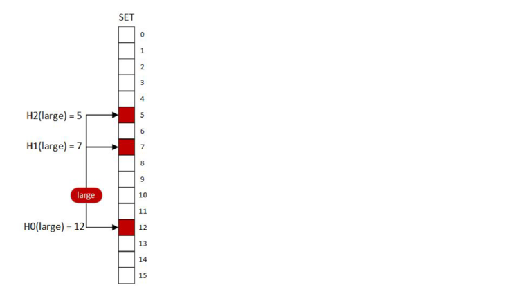
To insert “large” into the document, we’ll set bits five, seven, and twelve. To query for “large”, we’ll do the bitwise AND of those locations. That is, we’ll check to see if all three locations are 1. If any location is a 0, the result will be 0 (false) otherwise the result will be 1 (true). For any term we’ve inserted, the query will be 1 (true), because we’ve just set those bits.
In this series of diagrams, any bit that’s colored is a 1 and any bit that’s white is a 0. The red bits are associated with the term “large”.
1 (true) beacuse we’ve just set all the bits associated with the query.
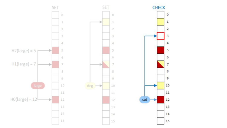
When we do the bitwise AND, we first look at bit three. Since bit three is a zero, we already know that the result will be 0 (false) before we look at the other bits and don’t have to look at bits ten and twelve.
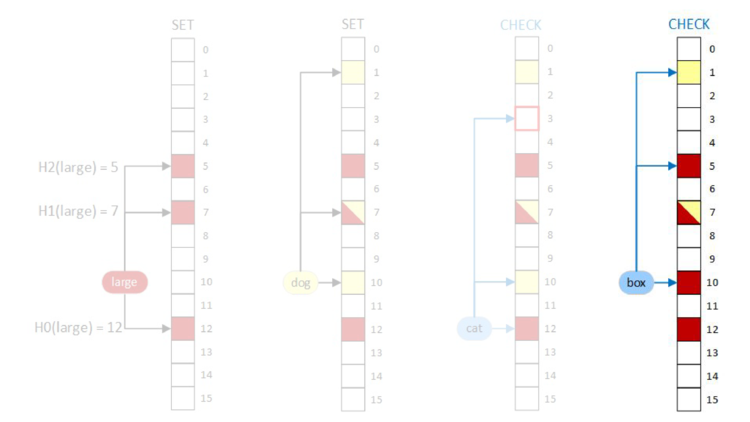
Even if we don’t insert this term into the document, the query shows that the term is in the document because those bits were set by other terms. We have a false positive!
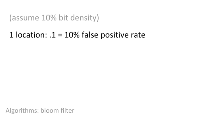
What’s the probability of a false positive if we hash to one location instead of three locations?
If the term is actually in the document, then we’ll set the bit, and if we do a query, since the bit was set, we’ll definitely return true, so there’s no probability of a false negative.
If the term isn’t in the document and we haven’t set the associated bit for this term because of this term, what’s the probability the bit is set? Because our bit desnity is .1, or 10%, the probability is 10%.
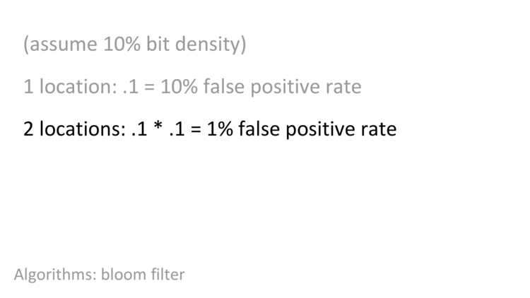
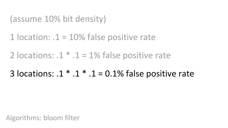
As we hash to more locations, if we don’t increase the size of the bit vector, the bit density will go up. Same amount of space, set more bits, higher bit density. So we have to increase the number of bits, and we have to increase the number of bits linearly. As we increase the number of bits linearly, we get an exponential decrease in the probability of a false positive.

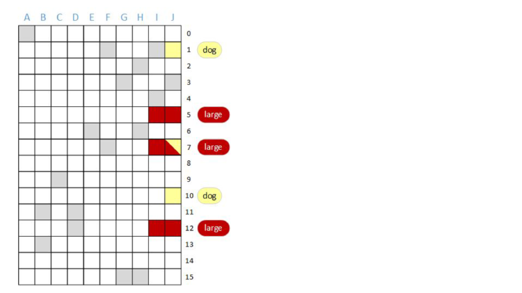
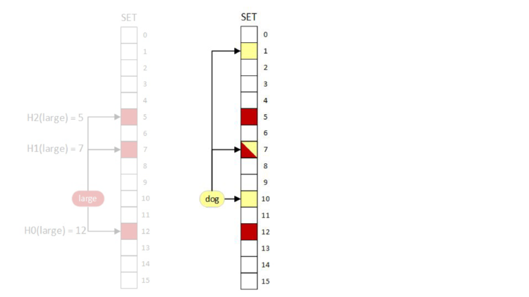
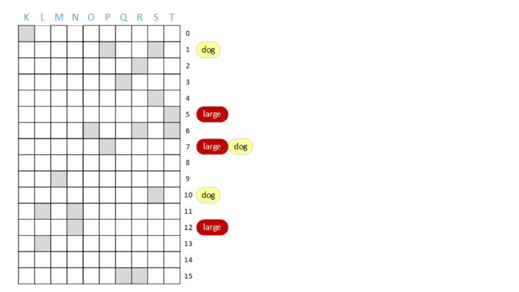
One thing we could do is have ten independent bloom filters. We know that we can have one bloom filter represent one document, so why not use ten bloom filters for ten documents?
If we’re going to do that, we might as well maintain the same mapping from terms to rows; that is, use the same hash functions for each column, so that when we do a query, we can do the query in parallel.
AND of some bits. Now, to do a query, we’ll do the bitwise AND of rows of bits.
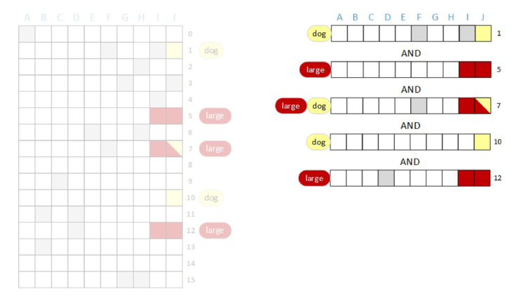
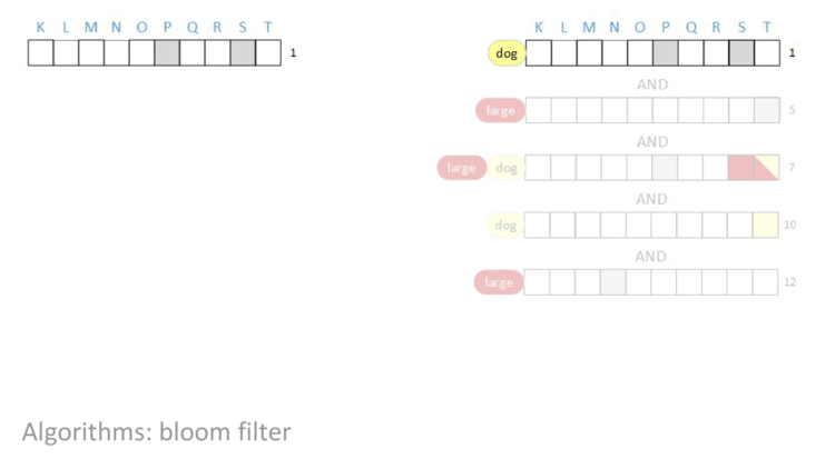
AND “dog”. As before, bits that are red are associated with the term “large” and bits that are yellow are associated with the “dog”. Additionally, bits that are grey are associated with other terms.
After we do the bitwise AND of all of the rows, the result will be a row vector with some bits set – those bits will be the documents that have both the terms “large” AND “dog”. We’re going to AND together rows one, five, seven, ten, and twelve and then look at the result.
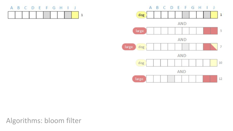
When we start, we have row one.
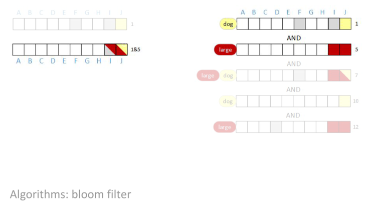
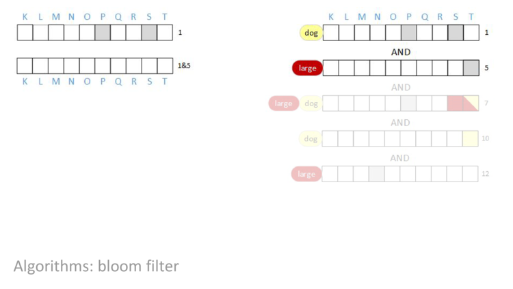
AND rows one and five together, we can see that bit F is cleared to zero.
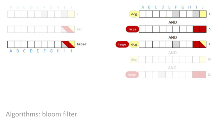
AND row seven into our result, nothing changes. Even though row seven has bit F set, an AND of a one and a zero is a zero, so the result in column F is still zero.
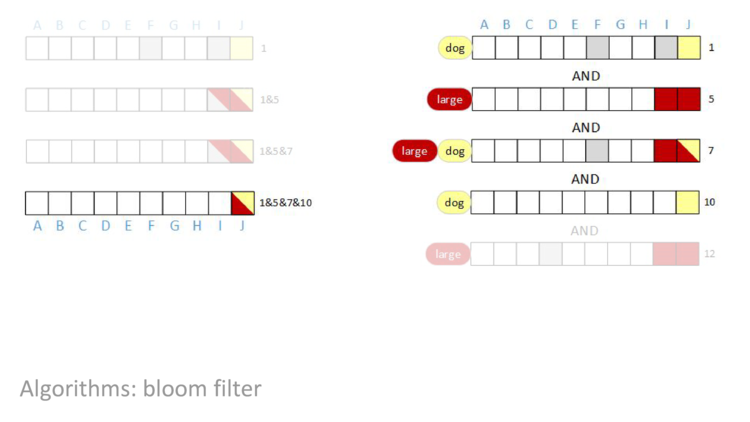
AND row ten in, bit I is cleared.
AND in the last row, nothing changes. The result of the query is that bit J is set. In other words, the query concludes that document J contains both the terms “large” AND “dog”, and no other document in this block contains both terms.
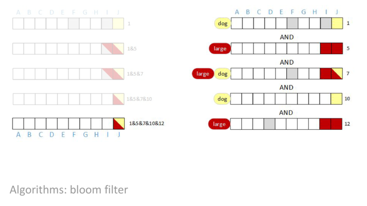
AND of rows one, five, seven, ten, and twelve.
AND in row five, all of the bits are zero! When that happened in the “cat” example we did on a single document, we could stop because we knew that the document couldn’t possibly contain the term cat because we can’t set a bit by doing an AND. This same thing is true here, and we can stop and return that the result is all zeros.
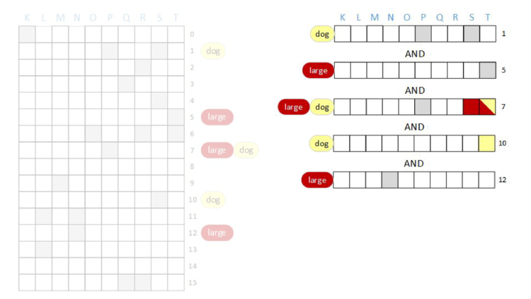
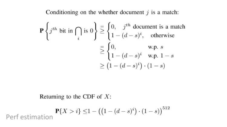
We’ll want to have a cost model for operations and then figure out what operations we need to do. For us, we’re doing bitwise ANDs and reading data from memory. Reading data from memory is so much more expensive than a bitwise AND that we can ignore the cost of the ANDs and only consider the cost of memory accesses. If we had any disk accesses, those would even slower, but since we’re operating in memory, we’ll assume that a memory access is the most expensive thing that we do.
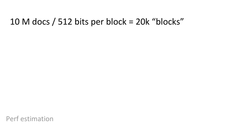
One bit of background is that on the machines that we run on, we do memory accesses in 512-bit blocks. So far, we’ve talked about doing operations on blocks of ten documents, but on the actual machine we can think of doing operations on 512 document blocks.
In that case, to get a performance estimate, we’ll need to know how many blocks we have, how many memory accesses (rows) we have per block, and how many memory accesses our machine can do per unit time.


AND “yellow” AND “dog”.

(large AND yellow AND dog) OR (golden AND retriever)
as well as other breeds of dogs that can be large and yellow.
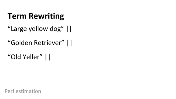
(large AND yellow AND dog) OR (golden AND retriever) OR (old AND yeller)
and in fact we might want to query for the phrase “old yeller” and not just the AND of the terms, and so on and so forth.
When do you this kind of thing, and add in personalization based on location and query history, simple seeming queries can end up being relatively complicated, which is how we can get queries of 100 rows.

Coming back to the histogram of the number of memory accesses per block, we can see that it’s bimodal.
There’s he mode on the right, where we do 14 accesses. That mode corresponds to our first multi-document example, where at least one document in the block contained the terms. Because at least one document contained all of the terms, we don’t get all zeros in the result and do all 14 accesses.
The mode on the left, which is smeared out from 3 on to the right, is associated with blocks like our second example, where no document contained all of the terms in the query. In that case we’ll get a result of all zeros at some point with very high probability, and we can terminate the query early.
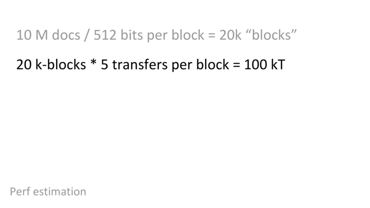
If we look at the average of the number of accesses we need for the left mode, it’s something like 4.6. On the right, it’s exactly 14. If we average these together, let’s say we get something like 5 accesses per query (just to get a nice, round, number).
There are some domains where that’s fine, but in web search, we spend a significant fraction of CPU time ranking the documents that match the query.
This is something BitFunnel can actually do faster than querying. If we think about how queries worked, they’re global, in the sense that each query looked at information for each document. But when we’re ingesting new documents, since each document is a column, that’s possible to do without having to touch everything in the index. In fact, since our data structure is, in some sense, just an array that we want to set some bits in, it’s pretty straightforward to ingest documents with multiple threads while allowing queries with multiple threads.
It’s possible to work through the math for this the way we did for querying, but again, in the interest of time, I’ll just mention that this is possible.
Between ranking and ingestion, in the configuration we’re running today, that uses about half the machine, leaving half for matching, which reduces our performance by a factor of two.

In our example, we had one bloom filter per document, which meant that if we had a query that only matched a single docucment, we’d have to examine at least one bit per document. In fact, we said that we’d end up looking at about five bits per document. If we use hierarchical bloom filters, it’s possible to look at a log number of bits per document instead of a linear number of bits per document.

Notice that some columns (B and D) have most or all bits set, and some columns (A and C) have few or no bits set. This is because different documents have a different number of terms.
Let’s say we sized the number of rows so that we can efficiently store tweets. Let’s say, hypothetically, that means we need fifty rows. And then a weird document with ten million terms comes along and it wants to hash into the rows, say, thirty million times. That’s going to set every bit in its column, which means that every query will return true. Many weird documents like this contain terms that are almost never queried, so the query should almost never return true, but our system will always return true!
Say we size up the number of rows so that these weird ten million term documents are ok. Let’s say that means we need to have a hundred million rows. Ok, our queries will work fine, but we still have things like tweets that might want to set, say, sixteen bits. We said that we wanted to use bloom filters instead of arrays to save space by hashing to reduce the size of our array, but now we have all of these really sparse columns that have something like sixteen out of a hundred million bits set.
To get around this problem, we shard (split up the index) by the number of terms per document. Unlike many systems, which only run in a sharded configuration when they need to spill over onto another machine, we always run in a sharded configuration, even when we’re running on a single machine.
Although there are other low level details that you’d want to know to run an efficient system, this is the only change that you absolustely have to take into account when compared to the algorithm I’ve described today.

“Search is simple”.
You’ve seen me describe an algorithm that’s used in production for web search. The algorithm is simple enough that it could be described in a thirty-minute talk with no background. However, to run this algorithm at the speed we’ve estimated today, there’s a fair amount of low-level implementation work. For example, to reduce the (otherwise substantial) control flow overhead of querying and ranking, we compile both our queries and our query ranking.
Additionally, even if this system were simple, this is less than 1% of the code in Bing. Search has a lot of moving parts and this is just one of them.
I went into some detail about bloom filters and didn’t talk about posting lists much, except to say that they’re standard. This might give the impression that bloom filters are categorically better than posting lists. That’s not true! I only didn’t describe posting lists in detail and do a comparison because state-of-the-art posting list implementations are tremendously complicated and I couldn’t describe them to a non-specialist audience in thirty minutes, let alone do the comparison.
If you do the comparison, you’ll find that when one is better than the other depends on your workload. For an argument that posting lists are superior to bloom filters, see Zobel et al., “Inverted files versus signature files for text indexing”.
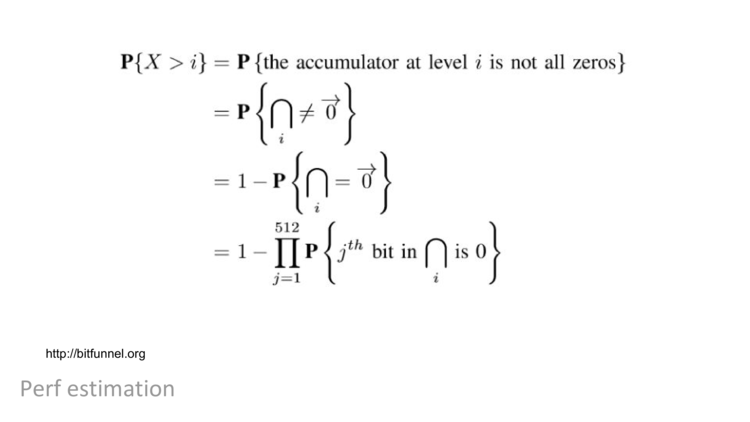
Today, we look at how an algorithm worked and estimated the performance of a system that took years to build. This was relatively straightforward because we were trying to calculate the average throughput of a system, which is something that’s amenable to back-of-the-envelope math. Something else that’s possible, but slightly more difficult, is to estimate the latency of a query on an unloaded system.
Something that’s substantially harder is estimating the latency on a system as load varies, and estimating the latency distribution.


Post original talk: also, thanks to Laura Lindzey, Larry Marbuger, and someone’s name who I can’t remember for giving me great post-talk feedback that changed how I’m giving the next talk.

Oh, yeah, I’m told you have to introduce yourself at these things. I’m Dan Luu, and I have a blog at danluu.com where I blog about the kind of thing I talked about here today. That is, I often write about performance, algorithms and data structures, and tradeoffs between different techniques.
Thanks for your time. Oh, also, I’m not going to take questions from the stage because I don’t know how people who aren’t particularly interested in the questions often feel obligated to stay for the question period. However, I really enjoy talking about this stuff and I’d be happy to take questions in the hallway or anytime later.
Some comments on the talk
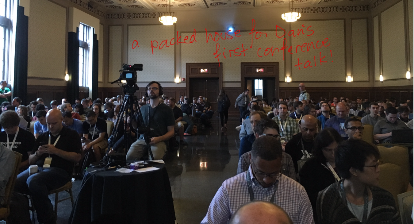
Phew! I survived my first conference talk.
Considering how early the talk was (10am, the first non-keynote slot), I was surprised that the room was packed and people were standing. Here’s a photo Jessica Kerr took (and annotated) while we were chatting, maybe five or ten minutes before the talk started, before the room really filled up:
During the conference, I got a lot of positive comments on talk, which is great, but what I’d really love to hear about is where you were confused. If you felt lost at any point, you’d be doing me a favor my letting me know what you found to be confusing. Before I run this talk again, I’m probably going to flip the order of some slides in the Array/Bloom Filter/BitFunnel discussion, add another slide where I explictly talk about bit density, and add diagrams for a HashMap (in the posting list section) and an Array (in the lead-up to bloom filters). There are probably more changes I could make to make things clearer, though!